Quantifying Option Versatility in T20s
How does one profile batters using their strong shots and zones?


To paraphrase my friend Kartikeya Date: in the longer formats batter plays the ball, while in T20 they play the field. As the common sense of the player pool in the shortest format rapidly imbibes fast-scoring, batters are looking for any and all advantages in their pursuit for boundaries. In the last 14 overs of an innings, this pursuit can take two forms: six-hitting or gap-finding. The former needs raw power and the ability to hit across lengths, whereas the latter takes finding the one undefended boundary with 5 fielders outside the inner ring.
The batter who can most successfully find that one gap in the boundary is one who possesses multiple shot options for the same ball. In my view, this is the future of T20 hitting and batter analyses. There have already been efforts to this end with the availability of wagon wheel and shot zone data. Most prominently, Arnav Jain’s all-encompassing app attempts to do this via an array of metrics.
The app has an intelligent wagon wheel that weights a batter’s wagon wheel by the rarity and relative SR of the zones accessed, a sector importance map, a nifty “360 score” that uses the angular variance of a batter’s wagon wheel spokes, and a simple but useful “field coverage”. The last metric asks how much of a batter’s runs can be covered using “n” outfielders — essentially telling you how many runs you leave undefended if you cover the batter’s “n” best zones. The app also paints an ideal field setup for a given batter. All these are extremely useful tools for both batters and fielding teams planning to thwart them.
Let’s look at this formally using the distribution of shot zones after weighting by line and length. Arnav’s aforementioned app already does this, but I want to explore a breakdown.
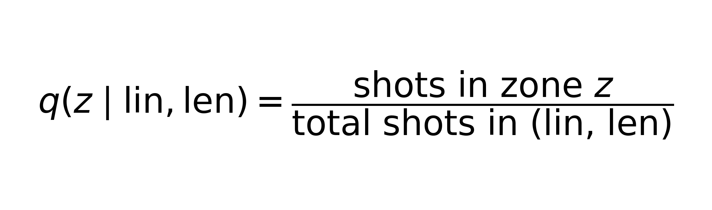
We want to compute the zone distribution of the “average” batter given the lines and lengths faced by our chosen batter. For now, let us consider only IPL 2025-26 data, counting only controlled scoring shots vs pace. We are considering 8 equal field zones. For each line (lin) and length (len) combination, we first construct the distribution (q) of wagon zones (z) for the pool of all batters:
Now, let’s take a batter and get the distribution of lines and lengths he has faced over the time period we are covering, and call this w(lin,len). Using this and q(z | lin,len), we construct a “counterfactual” distribution of zones:
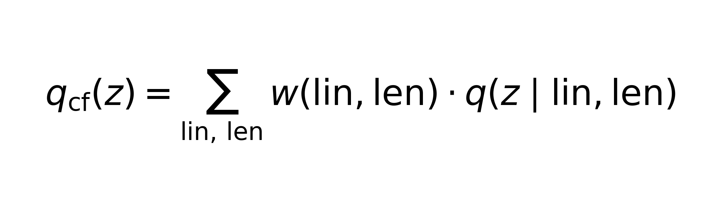
This is the distribution of zones if an average batter from our pool had faced the same lines and lengths. In a similar vein, we can compute the counterfactual runs-per-ball in each zone from the average batter facing the same lines and lengths:
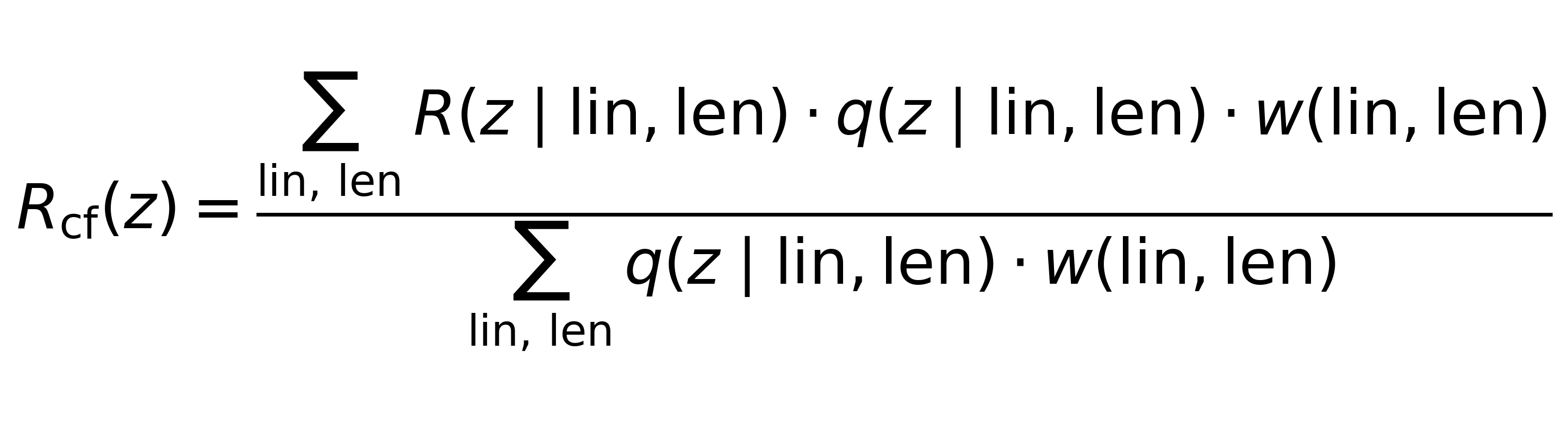
where R(z | lin,len) is the average runs per ball in zone “z” from balls of line “lin” and length “len”. R_cf(z) weighs this average run distribution by the proportion of balls faced by our chosen batter and the zones the ball would have gone to, if the average batter were facing them. Mathematically,
the w(lin,len) part tells you about the distribution of lines and lengths faced by the chosen batter;
the q(z | lin,len) part translates that to the wagon zone distribution that the average batter would have sent these balls to;
finally, the R(z | lin,len) tells you the average runs scored in each zone from each line/length combo.
We now have two “counterfactual” arrays: 1) the zone distribution of the average batter, and 2) the runs per ball in each zone from the average batter, both if they had faced the same balls as our chosen batter. These can be translated into a field plot like the one below, which shows a comparison on both these metrics for Abhishek Sharma.
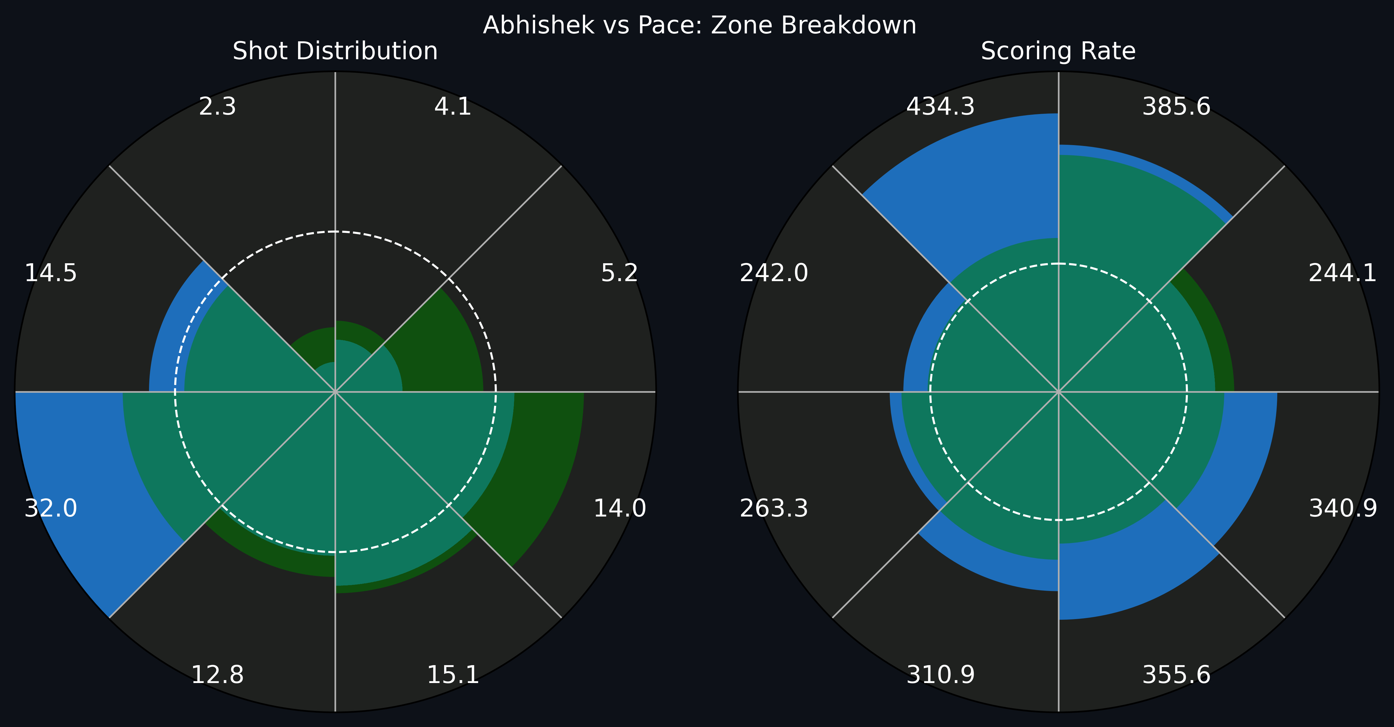
The left plot shows the % distribution of zones accessed, with blue showing Abhishek’s distribution, and green showing the average batter’s. All batters have been converted to RHB for this. You can see that Abhishek accesses the offside (two sectors on the left of the plot) more than the other batters given the ball areas he faces. The dashed circle in the left panel shows the 12.5% level: this would be the distribution if all zones were uniformly accessed. On the right you can see a similar comparison of his SR in different zones, with the white circle showing 200 SR just as a guide.
Below is the same plot for Vaibhav Sooryavanshi vs pace. As I discussed in my recent piece on ESPNcricinfo, he accesses the straight legside V much more often than other batters due to his unique backlift, bend of the back, and downswing.
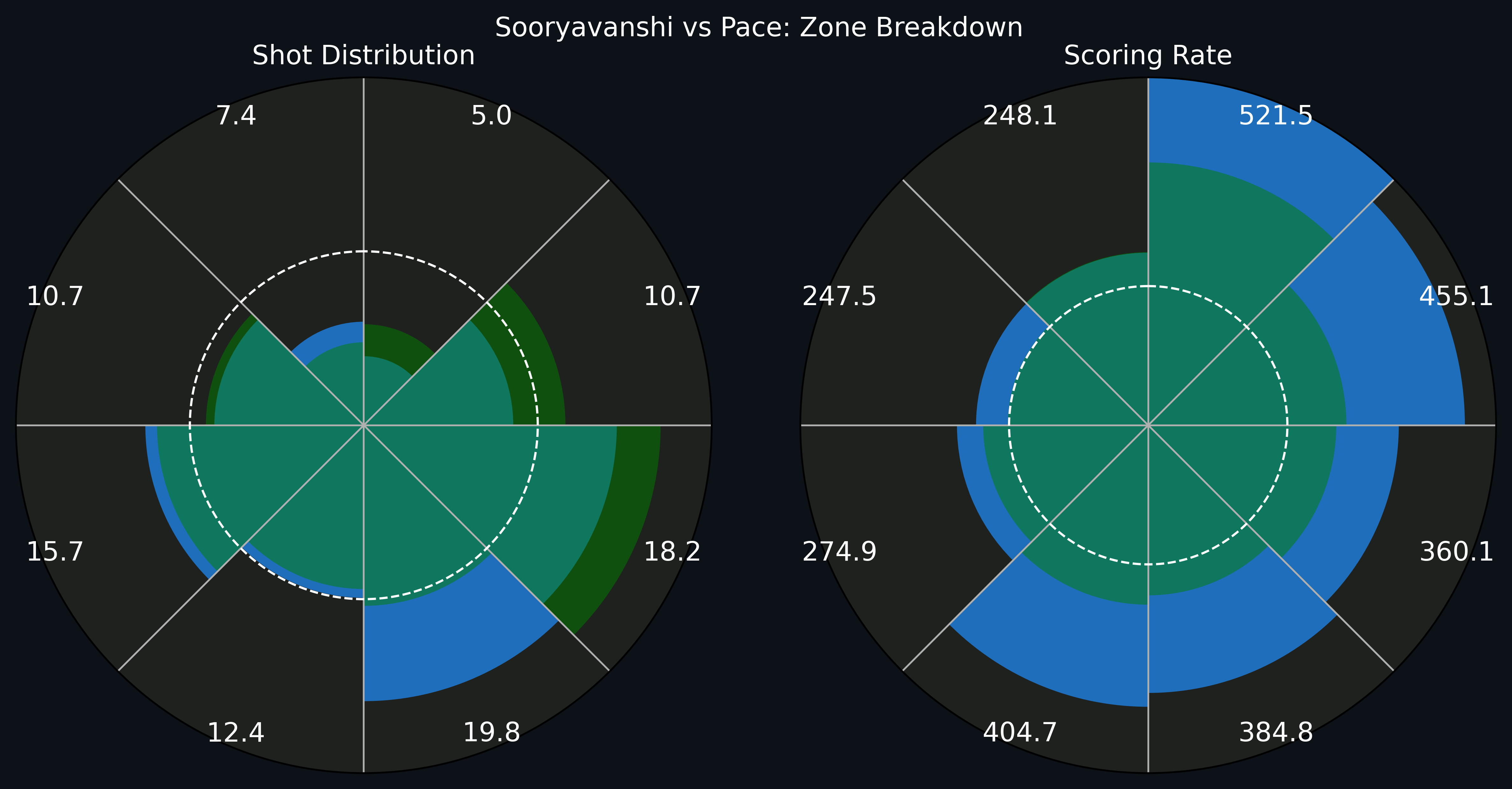
These figures can be a useful starting point for not just looking at strong and weak zones of batters, but also beginning to quantify the “diversity” of a batter’s shot options. For instance, in the two plots above, we can see that the bulk of both Abhishek Sharma’s and Sooryavanshi’s scoring is in 2-3 zones. Their SRs exceed the field’s SR by far, but their target areas are 3 zones. Compare this to Prabhsimran Singh’s zone breakdown, which seems to be more “evenly” distributed.
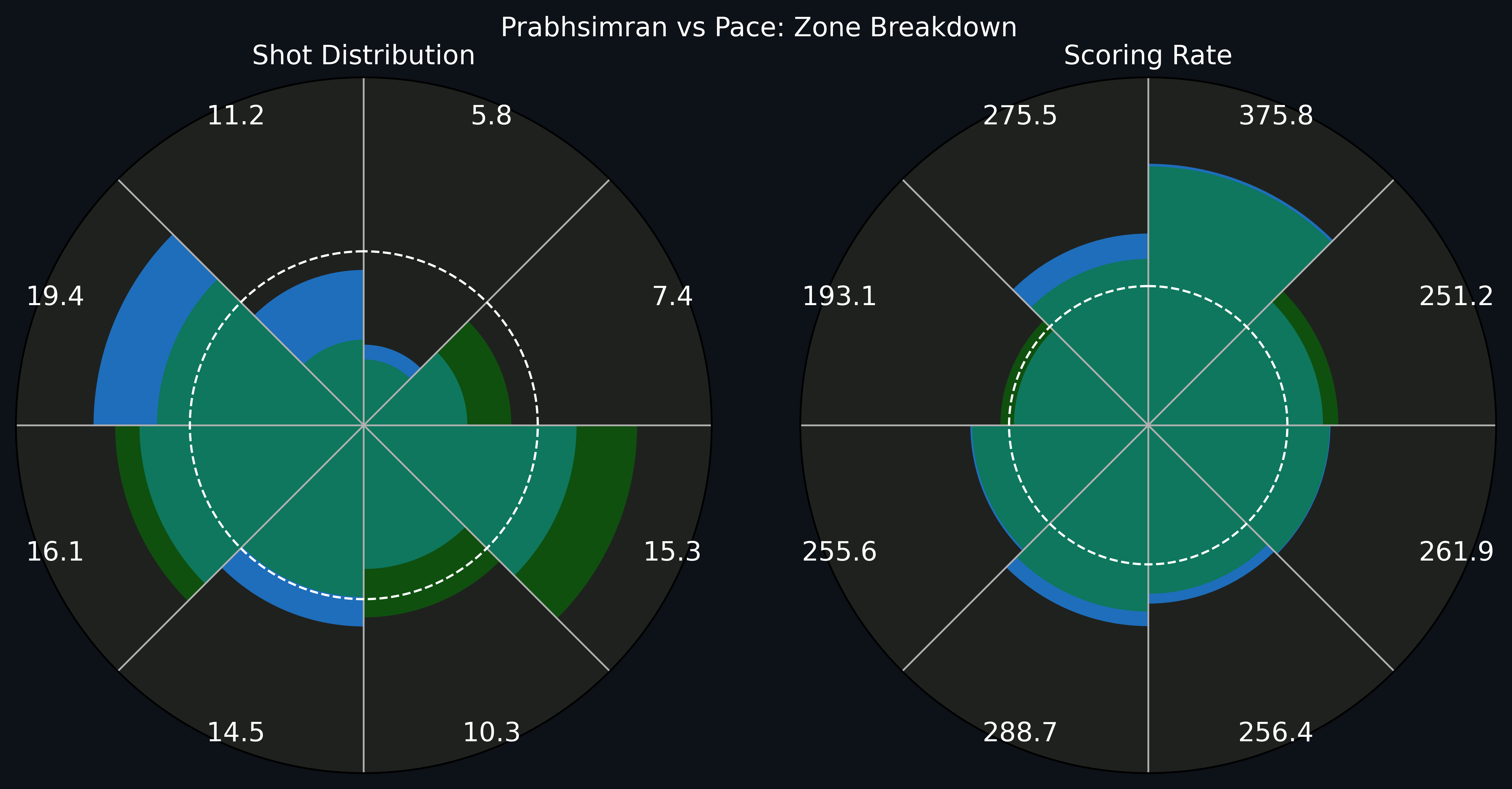
We are already getting a sense of different “styles” of batters: Abhishek and Sooryavanshi target fewer areas compared to Prabhsimran but they gun for maximising those areas. How can we formalise this notion?
Enter entropy. Entropy is commonly and colloquially called “disorder”, borrowing from its meaning in the thermodynamics / statistical physics sense. However, the same entropy plays a vital role in information theory, where it encodes the “ability to surprise” of a given distribution. A sharply lopsided distribution has low entropy. Let’s take a hypothetical batter who plays just one shot. When they play a shot, no opposing captain is surprised. Compare this to another hypothetical batter who plays 7 shots with equal probability: the fielding captain is unsure about which shot will be played, and is “surprised” more than they were facing the one-shot batter. The idea is that low-probability events possess more “information”. Entropy codifies this concept.
The formula for the entropy H(p) of a distribution p is
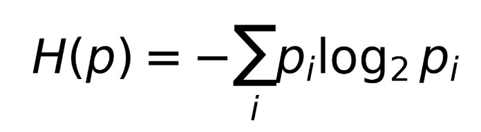
The entropy is is the expected “information” in a distribution, where the information (surprisal) is log(p).
(thanks to Omkar Walunj for pointing me in this direction as he was trying to replicate Cricviz’s “innovation” metrics)
Now, what does H(p) tell us about a batter? Let’s pivot to the distribution of shots for the batter. If the batter has just 2 shots, the entropy is low, since there are only two options, both with high probability. In contrast, if he has 8 shots, the entropy is high (the -log(p) term is high since the probability of each kind of shot is a smaller number). The 8-shot batter, one with more options, has a higher entropy. His shots can “surprise” the opposing team a lot more than the batter with just two shots.
So, the entropy of a batter’s shot distribution tells us the inherent unpredictability of a batter’s options.
A related number is the cross-entropy. The entropy H(p) told us about the average surprise of a batter’s shots, considering his own shot distribution. The cross-entropy, on the other hand, is
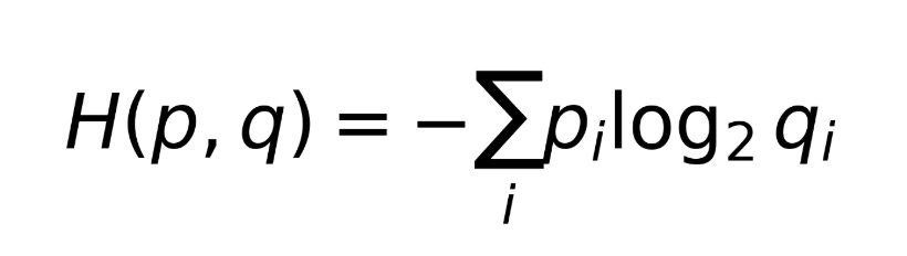
where p_i is the batter’s shot distribution and q_i is the average batter’s shot distribution. This quantity is weighing the batter’s shot options by the general rarity of shots. It can be increased by either of the two components of the product: if a batter plays a shot very often (high p_i), or/and if the shot is rare (low q_i).
Cross-entropy tells us the average unpredictability in a batter’s shots given we only know the average batter’s shot distribution. If I as a captain had studied only the average IPL batter, how much would this batter’s shots surprise me?
This kind of categorical cross-entropy is often used in deep learning applications when building multi-class classifiers.
A third, related quantity is the Kullback-Leibler Divergence (KL Divergence). This is simply the difference between the cross-entropy and self-entropy:
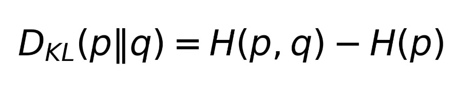
What does this tell us about a batter? A high D_KL means that the opposing captain stands to gain specific information about a particular batter by studying the batter’s patterns. In other words, the batter is unusual compared to the other batters in very specific ways. Doing your “homework” can give you substantial advantages in setting a field for a high D_KL batter. A low D_KL batter does not have any individual patterns in his shotmaking.
So, in summary:
High entropy H(p): batter’s own shotmaking is inherently unpredictable
High cross-entropy H(p,q): batter’s shotmaking is unusual compared to the average batter / the batter is difficult to set a field for if you have not studied him individually
High D_KL: specific homework can close the gap.
Let’s calculate this for IPL batters. We will do a more nuanced computation, since the shot hit is a function of line and length. For each batter, we will compute the entropy, cross-entropy and D_KL for each line and length combo, comparing to the average batter’s shot distribution for that line/length bin. We will then find the weighted mean of these three quantities for the batter, weighted by the number of balls faced by the batter.
Here is a plot of the D_KL (y axis) vs Entropy (x axis):
We have four quadrants here, divided using the medians of the entropy and D_KL. It’s worth exploring the cricketing meaning of each of these.
Top-right: high-entropy, high D_KL. These batters have a wide range of shots, and their shots are unusual compared to the other batters given the lines and lengths they face. Suryakumar Yadav and Rishabh Pant are typical of this kind of batter.
Top-left: low entropy, high D_KL. These batters have a small oeuvre of shots, but their shots are highly unusual compared to the average batter given the lines and lengths they face. They don’t have a lot of shots, but they need specific homework for field settings. Sunil Narine, Tim David and Ayush Mhatre are typical of this set: they have only a few shots (which they play well), but they can hit balls into their favourite areas from a variety of locations.
Bottom-left: low entropy, low D_KL. These batters have a small set of shots, like those in the top-left, but their shots are also “typically” distributed — close to the overall shot distribution given the balls they face. They do not need funky fields.
Bottom-right: high entropy, low D_KL. These batters have multiple options to the same ball, but their shot distribution is “usual”. These are classical batters and good pace hitters, as evidenced by the presence of Gill, Kohli and Rahul in there.
Here is a companion plot showing Entropy vs “score”. “Score” in this context is a weighted sum of the efficacy of each shot played by the batter for a line-length combination.
I would like to point out Vaibhav Sooryavanshi and Sunil Narine have low entropy (they have a small number of shots) but they execute them very well and have a high “score”. There are multiple ways to skin the cat when it comes to T20 hitting. Some, like Kohli and Gill, play a wide range of classical shots, sticking to conventional choices for the lines and lengths they face. Some, like Suryakumar play many shots but unconventionally. And some, like Sooryavanshi, play only a few shots, play them in zones like the average batter would, but don’t care about the field too much, executing them perfectly.
This was just a little idle pondering and Sunday doodling, and I don’t know how useful this can be, but I liked this as an academic tool to explore the “types” of batters by their field access. Batter profiling is mostly done by line/length outcomes, but field access is extremely important in T20s, and I hope this kind of analysis can enter the broader discussion. We do not possess fieldset data, which I think is a crucial component of T20 analysis going forward. While we wait for that, I think cricket analytics should start building the machinery to profile batters via their shots. After all, batter intent is the dominant determinant of a ball’s outcome in T20s (~65%).